4. A quantification of Energy fluxes.
Key concepts: Solar constant. Earth Energy Imbalance (EEI). Our oceans act as heat sinks and carbon sinks. Radiative Forcing. MCB could cool our planet by 0.4 C. Ocean degasification and acidification. The complex role of clouds and aerosols.
The sun’s energy reaches Earth as shortwave radiation (check out Chapter 2, GHGs absorb IR radiation emitted by Earth). Flows – such as energy flow per second – are often referred to as fluxes. The sun’s flux is remarkably constant. When measured per square meter of radiated surface, it has a value of approximately 1,361 W/m2, and this value is known as the solar constant. The solar constant is calculated based on Earth’s cross-sectional area as a sphere. Since the surface area of a sphere is four times its cross-sectional area (4), the globally and yearly averaged Top of Atmosphere (TOA) incoming solar radiation is approximately a quarter, ~340 W/m2.
How constant is the solar constant? Very constant. Our sun has an 11-year solar activity cycle. The lowest observed solar constant of 1,360.3 W/m2 occurred during the minimum between the 23rd and 24th solar cycle (2008-2009). The highest observed solar constant of 1362.0 W/m2 occurred during the solar maximum of cycle 24, around 2014. A slightly larger variation of 3% is caused by Earth’s elliptical orbit around the Sun. This variation is regular, predictable and accounted for in weather and climate models. As we shall read further on, even though these changes are small, they can still have subtle effects on Earth’s climate system, particularly when considering long-term trends.
Let us now consider energy fluxes under the assumption of solar radiation balance. As we learned in Chapter 2, to avoid global warming, this shortwave solar “Energy In” of ~340 W/m2must be balanced by a similar ~340 W/m2 terrestrial radiation “Energy Out”.
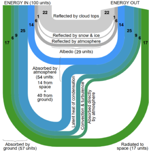
Source: Wikimedia Commons, ‘Earth heat balance Sankey diagram’. Licensed under CC BY-SA 3.0; adapted by Refreeze the Arctic Foundation.
[Ref.:https://upload.wikimedia.org/wikipedia/commons/2/29/Earth_heat_balance_Sankey_diagram.svg; updated ]
In the above Sankey diagram, of the ~340 W/m2 of shortwave solar radiation received by Earth, around 29 units (29% or ~100 W/m2) in this example are directly reflected back to space as shortwave radiation: 22 from the top of clouds, 1 from snow and ice-covered areas, and 6 by other parts of the atmosphere (thanks to Earth’s reflecting white surfaces, it’s albedo). The 71 remaining units (~240 W/m2) are called Absorbed Solar Radiation (ASR): 14 units are absorbed within the atmosphere and 57 by the Earth’s surface. Of these, 17 units are again directly radiated to space, but now in the form of longwave blackbody IR radiation. The rest, 40 units, is eventually absorbed by the atmosphere by various mechanisms and ultimately re-emitted to space as longwave blackbody IR radiation. These 71 units of longwave blackbody IR radiation are called Outgoing Longwave Radiation (OLR). We visited the spectra of the ASR and OLR in Chapter 2. There is solar radiation balance when ASR = OLR.
Let us now consider a situation where there is solar radiation imbalance, and specifically where ASR > OLR, which is today’s situation.
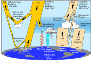
Source: Ocean Wiki, ETH Zurich. Authors: Stephanie Remke, Andreas Hagmann, Peter Stricker. Licensed under CC BY-SA 4.0; adapted by Refreeze the Arctic Foundation.
[Ref.: Ocean Wiki The Earth’s Energy Budget; Authors: Stephanie Remke, Andreas Hagmann, Peter Stricker; updated ]
The figure above illustrates the average energy fluxes of Earth’s energy budget, indicated by arrows, as recorded amongst others by satellites over several decades.
In the arrows figure, the atmospheric window appears in the OLR as 40 W/m2. CO2 emissions narrow this window (check out Chapter 2), driving the increase in EEI. Also, as Earth warms, atmospheric water content (clouds) rises by 7% per degree of warming, acting as a potent greenhouse gas and creating a strong positive feedback loop.
In the middle is the incoming short-wave solar constant of 340 W/m2. Earth’s albedo reflects 76.9+23=99.9 W/m2 (upward arrow on the left) shortwave radiation directly back into space (implying a reflection of 29%). The ASR is 340-99.9 = 240.1 W/m2, whilst the OLR (upward arrow on the right) is 239 W/m2. ASR > OLR. The seemingly tiny excess energy absorbed by Earth of ~1.1 W/m2 (240.1 – 239) is called the Earth Energy Imbalance (EEI). It is recorded in the bottom middle of the arrows figure as “net absorbed”. It is the EEI which causes global warming. The EEI is dynamic. It has increased from approximately ~0.5 W/m2 in the 1970s to ~1.1 W/m2 today (as measured by satellites).

Source: K. von Schuckmann et al., ‘Heat stored in the Earth system’, Earth System Science Data 12, 2013-2041 (2020). Open access under CC BY 4.0.
Tiny it may seem, but since the 1960s, the EEI accounted for ~400 Zettajoules additional energy absorbed by planet Earth in the form of heat, see the above figure (dotted lines = uncertainty interval). Humanity’s yearly average primary energy production over the last 40 years (check out Chapter 11, Economic cost, Proposition 7) was roughly 400 Exajoules. 400 ZJ/400EJ = 1000. Therefore, since the 1960s, due to the seemingly tiny radiation imbalance, Earth has stored a thousand years’ worth of human primary energy production as heat, mostly in our oceans. Marine biodiversity is suffering accordingly, with coral reefs close to extinction.
It is now useful to introduce Radiative Forcing (RF). RF is a scientific concept used to measure changes in Earth’s energy balance caused by external factors such as greenhouse gases, aerosols, surface reflectivity, and solar output. It is defined as the change in net radiative energy, equalling downward flux – incoming energy into the Earth system – minus upward flux – outgoing energy leaving it back to space. RF is measured in watts per square meter and is typically evaluated at the tropopause or top of the stratosphere and averaged globally. A planet in radiative equilibrium has zero RF and a stable equilibrium temperature.
RF cannot be directly measured but is calculated using physical principles and atmospheric data. According to the IPCC, human activities caused a RF of about +2.72 W/m2 in 2019 compared to 1850 (+ indicating warming), primarily due to increased greenhouse gas concentrations, partly offset by cooling from aerosols. Carbon dioxide is the largest contributor, with a 50% increase since 1850 causing about +2.16 W/m2 of forcing; a future doubling – the definition of climate sensitivity – would lead to about +3.71 W/m2 (see Chapter 1, Climate Sensitivity).
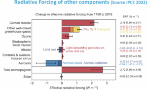
Source: IPCC Sixth Assessment Report (AR6), Working Group 1: The Physical Science Basis (2022).
Overall, five major greenhouse gases account for about 96% of the RF since the industrial revolution.
Radiative Forcing (RF) and Earth’s Energy Imbalance (EEI) are closely linked but describe different stages of the climate system’s response to a disturbance.
RF represents the initial change in Earth’s energy balance caused by external drivers such as increased CO2. This forcing creates a mismatch between incoming absorbed solar radiation (ASR) and outgoing longwave radiation (OLR), producing a positive EEI – meaning Earth absorbs more energy than it emits (also check out Chapter 2, Greenhouse gases absorb IR radiation emitted by Earth).
In response to RF, excess energy is stored mainly in the oceans, which warm slowly due to their large heat capacity. As ocean and atmospheric temperatures rise, OLR increases, progressively reducing the EEI. In theory, a temperature rise of about 1.1 °C would be sufficient to offset a radiative forcing of +3.71 W/m2 from a CO2 doubling if no positive feedback loops were present. However, positive feedback loops —especially involving water vapour and clouds—amplify the warming, making the expected equilibrium response closer to about 3 °C (see Chapter 1. How it all begun: climate sensitivity). Clearly, if climatic tipping points are crossed, established relationships may break down, and past correlations or responses can no longer be assumed to hold.
Because ocean warming is slow, the climate system cannot adjust instantaneously to rising RF. As a result, the atmosphere has not yet warmed enough to fully restore radiative balance, which is why Earth currently exhibits a positive EEI of ~1 W/m2.
RF therefore also predicts future equilibrium temperature increases. For example, a RF of +2.72 W/m2 implies a future equilibrium temperature of 3.0*2.72/3.71 = ~2.2 °C warming. Please note that RF is dynamic, and probably higher today than it was in 2019.
Using the same logic, if MCB aims to increase Earth’s albedo by 0.5 W/m2, MCB would cool the Earth by 3.0*0.5/3.71 = ~0.4 °C. Only field experiments can give better answers regarding MCB’s cooling potential.
As usual, science surprises us with its answers. In this case, minute changes in heat fluxes compared to ASR and OLR have a profound influence on our climate. And the existence of the atmospheric window makes our climate particularly sensitive to changes in atmospheric CO2 concentrations (see Chapter 2, Atmospheric Window).
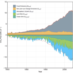
Source: P. Friedlingstein et al., ‘Global Carbon Budget 2019’, Earth System Science Data 11, 1783-1838 (2019). Open access under CC BY 4.0.>
Higher ocean temperatures are also a worry as oceans act as a large CO2 sink too (the CO2 flux on the y-axis is expressed as Gt C(arbon) per year, as opposed to the more usual Gt CO2 per year). In principle, liquids release dissolved gases at higher temperatures. Could the warming of seawater cause the oceans to release stored CO2 back into the atmosphere, a process called degassing?

Source: NOAA PMEL Carbon Program. Public domain. https://www.pmel.noaa.gov/CO2 /story/Ocean%20Acidification
The oceanic reality is vastly more complex, with absorbed CO2(aq) chemically reacting to form carbonic acid (H2CO3), which then acidifies the oceans:
CO2(aq) + H2O ↔ H2CO3 (1)
H2CO3 ↔ HCO3– + H+ (2)
HCO3– ↔ CO32- + H+ (3)
Carbonate ions can further react to form calcium- or other carbonates.
And seawater buffers the concentration of CO2 : CO2(aq) + CO32- + H2O → 2HCO3– (4)
Furthermore CO2(g) in the atmosphere and CO2(aq) dissolved in seawater are also in equilibrium. And we know that CO2(g) is increasing due to GHG emissions. But still. We should be alert to signs of ocean degasification.
It is important to clarify that ocean acidification does not imply that oceans are becoming acidic, but rather that they are experiencing a decrease in alkalinity. For those interested in the chemistry:

Source: Compiled by Refreeze the Arctic Foundation, adapted from Wikipedia articles ‘Bjerrum plot’ and ‘pH’. Licensed under CC BY-SA 4.0.
One can make two additional remarks about energy fluxes.
The first remark relates to the complex role of clouds in the Earth’s energy budget. Clouds reflect a substantial amount of incoming solar energy back to space (29% in the Sankey diagram). But being made up primarily of H2O (water vapour), they also absorb massive amounts of terrestrial infrared radiation, radiating it back in all directions, including back to Earth – the back radiation – and warming its surface:

Source: Colorado State University CMMAP (NSF-funded educational resource). https://hogback.atmos.colostate.edu/cmmap/learn/clouds/climate2.html
The total back radiation is no less than 330-340 W/m2, almost equivalent to the incoming solar radiation of 340.4 W/m2!
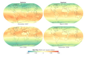
Source: NASA images via FLASHFlux team, NASA Langley Research Center. Caption by Rebecca Lindsey. Public domain (NASA). https://science.nasa.gov/earth/earth-observatory/seasonal-changes-in-global-net-radiation-35555/
The second remark relates to averages. In the above discussions, we treated heat fluxes as averages (as recorded by satellites in thousands of measurements over decennia), but their distribution over the planet and over the seasons is very uneven, leading to very different local climatic outcomes (green: absorbs, yellow: in balance, red: emits).
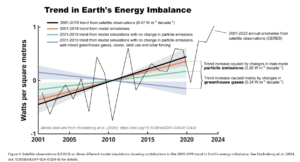
Source: Hodnebrog et al. (2024), Communications Earth & Environment. Licensed under CC BY 4.0. https://doi.org/10.1038/s43247-024-01324-8
Recently, Cicero published a graph showing that the rising trend in the EEI (black line) is actually made from 2 components: (i) an increase of the EEI due to greenhouse gas emissions of 0.34 W/m2 per decade but also (ii) a decrease in the emission of man-made sunlight-reflecting particles thanks to better environmental legislation such as removing sulphur from ship exhausts. This decrease has unintentionally increased the EEI by a substantial 0.20 W/m2 per decade (orange vs green line), strongly contributing to global warming.
We might have underestimated the role of aerosols in Earth’s energy budget. (https://doi.org/10.1038/s43247-024-01324-8).
The EEI dips substantially in 2011. This dip is attributed to the concurrence of a La Niña event (increased cloud cover, cooler equatorial Pacific ocean surface waters), the eruptions of Sarychev Peak in 2009 (Kuril Islands) and Nabro in 2011 (Eritrea), the latter one of the largest SO2-emitting events of the decade, a deep solar minimum between cycle 23 and 24, consistently high industrial aerosol emissions in Asia, and more heat being absorbed by the deep ocean. This latter process is consistent with the idea that short-term cooling events don’t mean global warming has stopped—just that the heat is going somewhere else temporarily.